Theoretical Background: Radar Remote Sensing Fundamentals
1 Introduction: The Active Microwave Perspective
Radar (Radio Detection and Ranging) remote sensing represents a fundamentally different approach to Earth observation compared to optical and infrared methods. While passive optical sensors rely on reflected sunlight, radar systems actively transmit microwave radiation and measure the backscattered signal (Lillesand, Kiefer, and Chipman 2015). This active nature, combined with the long wavelengths of microwave radiation (ranging from millimeters to meters), provides unique capabilities that overcome many limitations of passive optical remote sensing.
While passive microwave radiometers also exist—measuring naturally emitted thermal microwave radiation from the Earth’s surface—this chapter focuses exclusively on active radar systems. Passive microwave sensors operate similarly to thermal infrared sensors but at longer wavelengths, providing information primarily about surface temperature, soil moisture, and atmospheric water content (Ulaby and Long 2013). However, active radar systems offer distinct advantages: they provide their own controlled illumination, achieve much finer spatial resolution through coherent signal processing, and enable measurement of surface geometric and structural properties through analysis of backscattered signals.
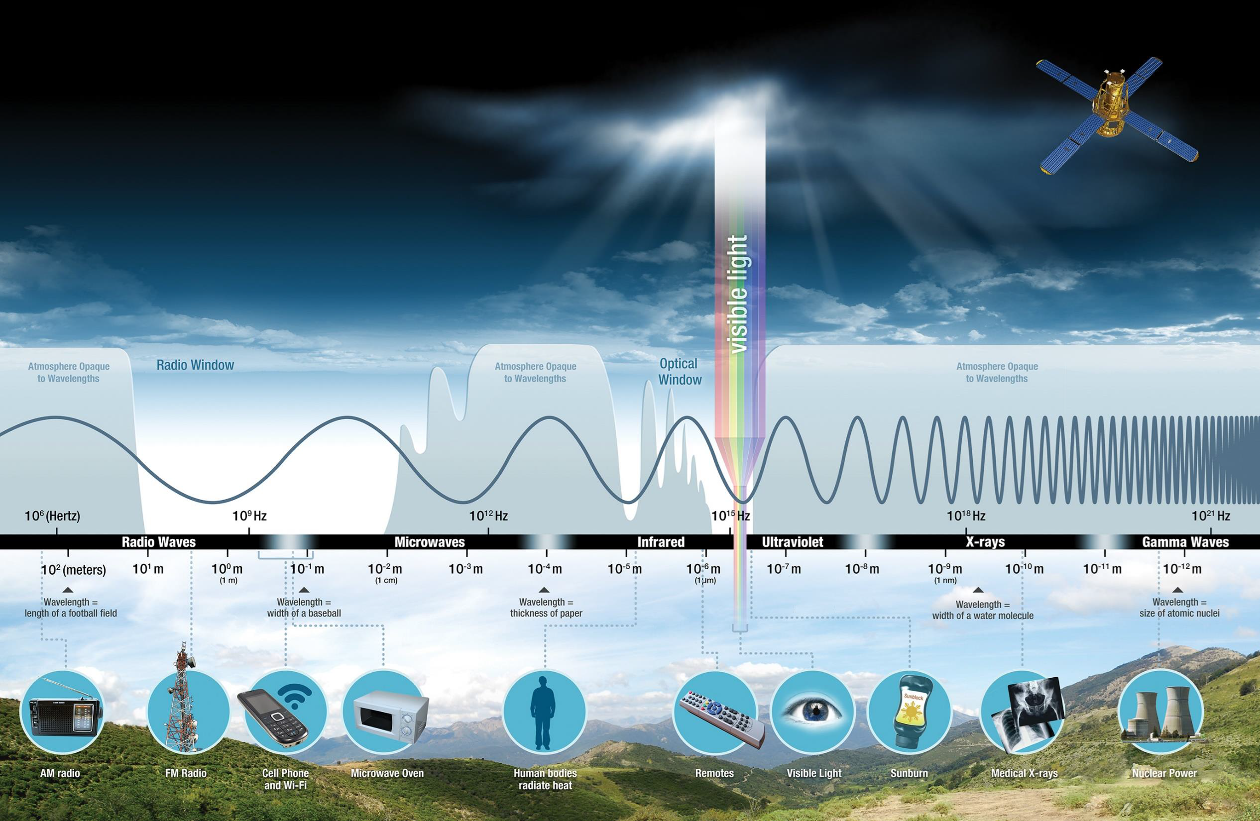
The electromagnetic spectrum shows that microwave radiation occupies the region between radio waves and infrared radiation, with wavelengths ranging from approximately 1 mm to 1 m (Figure 1). Within the atmosphere, specific wavelength regions—called atmospheric windows—allow electromagnetic radiation to propagate with minimal attenuation. The microwave region features broad atmospheric windows that enable radar signals to penetrate clouds, fog, rain, and darkness, providing all-weather, day-and-night imaging capabilities (Ulaby and Long 2013).
Three fundamental advantages distinguish radar from optical remote sensing:
- Active illumination: Radar provides its own energy source, enabling observations regardless of solar illumination and at any time of day or night (Henderson and Lewis 1998)
- Cloud penetration: Microwave radiation passes through clouds, smoke, and atmospheric moisture that block optical sensors (Woodhouse 2017)
- Surface penetration: Longer radar wavelengths can penetrate vegetation canopies and even soil or ice surfaces, revealing subsurface structures and volume properties (Ulaby and Long 2013)
These capabilities make radar particularly valuable for forest monitoring, where cloud cover often obscures optical observations in tropical and temperate regions, and where information about forest structure extends throughout the three-dimensional canopy volume rather than just the top surface visible to optical sensors.
2 The Importance of Forests: Context for Radar Applications
Understanding why radar remote sensing matters for forest monitoring requires first appreciating the critical role forests play in Earth’s systems (Figure 2). Forests are crucial for regulating energy, water, and carbon balance, covering 31% of Earth’s solid surface and 43% of the European Union’s area (Bonan 2008). They represent Europe’s most important renewable source of biomass and deliver livelihoods for 1.6 billion people globally (FAO 2020). Forests provide habitat for the vast majority of terrestrial plant and animal species, making their monitoring essential for biodiversity conservation (FAO and UNEP 2020).

Traditional optical remote sensing faces significant challenges in forest environments. Dense tropical forests occur in regions with persistent cloud cover, limiting optical data acquisition to rare cloud-free windows. Even in temperate zones, seasonal cloud patterns can prevent optical observations for weeks or months (Woodhouse 2017). Moreover, optical sensors primarily detect the uppermost canopy layer, providing limited information about understory structure, stem volume, or subsurface moisture (Kasischke et al. 2019).
Radar overcomes these limitations by penetrating clouds and, depending on wavelength, penetrating into and through vegetation canopies. The degree of penetration depends on the radar wavelength: shorter wavelengths (X-band, C-band) primarily interact with leaves and small branches, while longer wavelengths (L-band, P-band) penetrate deeper into canopy structure and interact with larger branches and stems (Figure 8). This wavelength-dependent penetration enables estimation of forest structural parameters including canopy height, biomass, and vertical profile that remain inaccessible to optical methods (Le Toan et al. 2011).
3 Why Microwave Radiation?
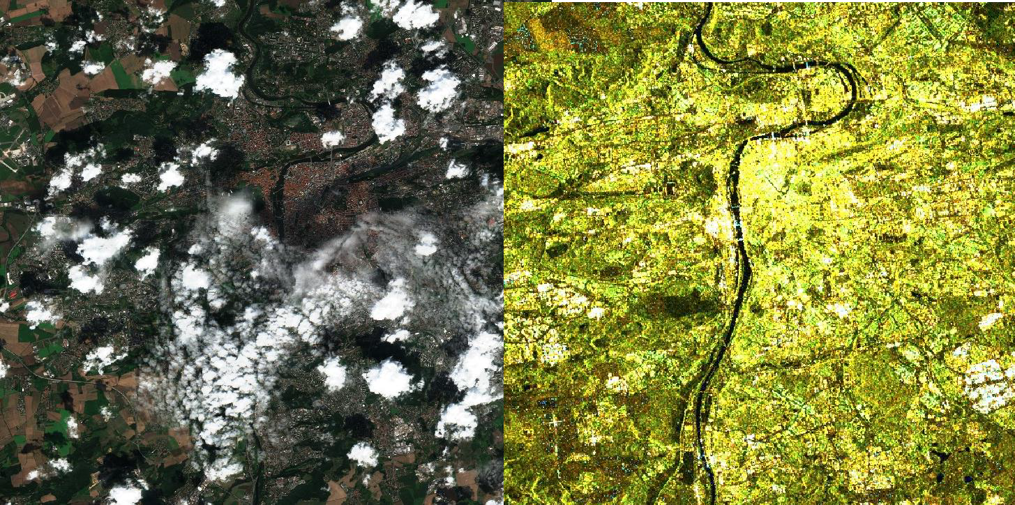
The choice of microwave frequencies for radar remote sensing stems from fundamental physical principles governing electromagnetic wave propagation and interaction with Earth’s atmosphere and surface. Figure 3 illustrates the dramatic difference between optical and radar imaging: the left image shows an optical view dominated by clouds obscuring the surface, while the right image demonstrates radar’s ability to see through these clouds to reveal underlying landscape features.
The physical basis for this capability lies in the relationship between electromagnetic radiation wavelength and atmospheric interaction. Figure 4 shows the spectral distribution of solar radiation (Sun’s energy at 6000 K) and Earth’s thermal emission (Earth’s energy at 300 K) across the electromagnetic spectrum. The critical observation is that between these natural emission peaks lies a region of minimal natural radiation—the microwave gap (Ulaby and Long 2013).
In this microwave region, there is insufficient natural radiation for passive sensing, necessitating active illumination. However, this same region features excellent atmospheric transmission—electromagnetic waves at microwave frequencies experience minimal absorption by atmospheric water vapor, oxygen, and clouds (Woodhouse 2017). This atmospheric window extends from approximately 1 cm to 1 m wavelength, encompassing the standard radar bands used for remote sensing.
The microwave region offers additional advantages beyond cloud penetration:
- Reduced atmospheric scattering: Unlike visible light, microwave radiation experiences minimal Rayleigh scattering from air molecules and aerosols (Henderson and Lewis 1998)
- Minimal ionospheric effects: At frequencies above ~1 GHz (wavelengths shorter than ~30 cm), ionospheric refraction becomes negligible for space-based systems (Meyer, Nicoll, and Doulgeris 2019)
- Weather independence: Radar imaging quality remains consistent regardless of solar illumination, precipitation (except very heavy rain at shorter wavelengths), fog, or smoke (Woodhouse 2017)
These properties make radar particularly valuable for operational applications requiring guaranteed data acquisition, such as disaster response, military reconnaissance, and continuous monitoring programs where temporal gaps are unacceptable.
4 Side-Looking Radar Geometry
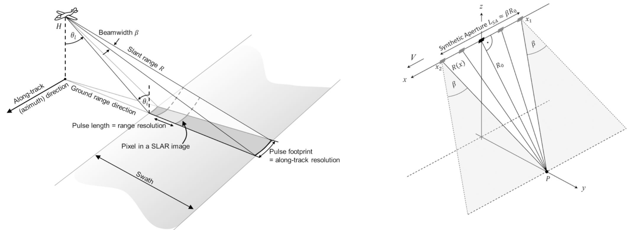
The fundamental geometry of radar imaging systems differs profoundly from optical sensors. While optical sensors typically observe directly beneath the platform (nadir-looking), imaging radar systems employ a side-looking geometry that is essential to their operational principle (Figure 5). This geometric arrangement creates both unique capabilities and specific challenges that shape how radar data must be acquired and interpreted.
4.1 Geometric Parameters
The side-looking configuration is defined by several critical geometric parameters (Henderson and Lewis 1998):
- Slant range (R): The direct distance from the antenna to a target on the ground
- Ground range: The horizontal distance from the point directly beneath the antenna to the target
- Look angle (θ): The angle between nadir (vertical) and the line from antenna to target
- Incidence angle (θi): The angle between the incident radar beam and the perpendicular to the local surface (normal)
- Depression angle: The angle between horizontal and the radar beam
- Beamwidth (β): The angular extent of the transmitted radar pulse
The relationship between these parameters determines the spatial resolution and geometric distortions in radar images. The range resolution—the ability to distinguish separate targets along the line of sight—is determined by the radar pulse length:
\[R_{res} = \frac{c \tau}{2 \sin \theta}\]
where c is the speed of light, τ is the pulse duration, and θ is the look angle (Woodhouse 2017). The factor of 2 appears because the radar signal must travel to the target and back.
The azimuth resolution—the ability to distinguish targets along the direction of platform motion—depends on the antenna aperture length (L) and slant range (R):
\[A_{res} = \frac{\lambda R}{L}\]
For real aperture radar systems, achieving fine azimuth resolution requires either very long antennas or short ranges. Synthetic Aperture Radar (SAR) overcomes this limitation by synthesizing a long antenna aperture through platform motion, achieving azimuth resolution given by (Cumming and Wong 2005):
\[A_{SAR} = \frac{L}{2}\]
remarkably independent of range and wavelength. This makes SAR the dominant technology for space-based radar remote sensing, enabling meter-scale resolution from satellite altitudes of hundreds of kilometers.
4.2 Why Side-Looking?
The side-looking geometry is not merely a design choice but a fundamental requirement for imaging radar systems (Henderson and Lewis 1998). If a radar looked straight down (nadir), all targets at equal range would return echoes simultaneously, making it impossible to distinguish their positions laterally. The side-looking geometry resolves this ambiguity by ensuring that targets at different ground positions have different slant ranges, enabling their spatial separation in the resulting image.
Additionally, the oblique illumination creates shadows and highlights topographic features, enhancing the interpretability of terrain and surface structure. The specific choice of look angle represents a trade-off: steeper angles (closer to nadir) reduce geometric distortions and shadow areas but decrease sensitivity to surface roughness, while shallower angles (more oblique) maximize roughness sensitivity but increase geometric distortions and shadowing (Woodhouse 2017).
For vegetation and forestry applications, moderate incidence angles (typically 20-40°) provide an optimal balance: sufficient penetration into canopy structure, sensitivity to volume scattering from branches and leaves, and manageable geometric distortions (Kasischke et al. 2019).
5 Surface Geometry and Scattering Mechanisms
The interaction between radar waves and Earth’s surface is fundamentally governed by the surface’s geometric and dielectric properties. Unlike optical remote sensing, where surface reflectance is largely determined by chemical composition and pigments, radar backscatter is dominated by structural geometry—the size, shape, orientation, and arrangement of scattering elements—and by dielectric constant, which is primarily controlled by moisture content (Ulaby and Long 2013).
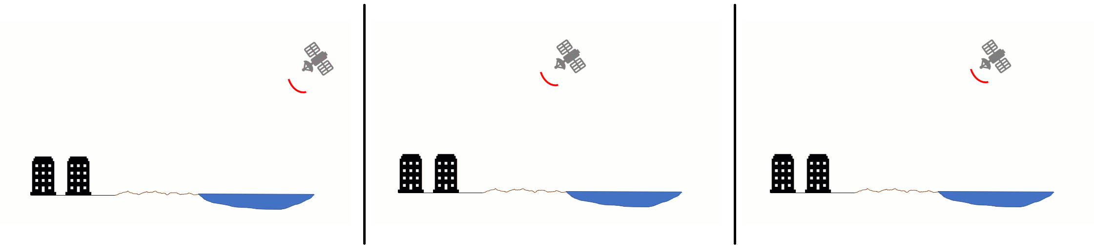
Figure 6 illustrates a fundamental principle: surface geometry matters profoundly for radar backscatter. The same objects (buildings, water body, terrain) illuminated from different directions produce dramatically different backscatter patterns. This angular dependence stems from the coherent nature of radar radiation and the resulting interference patterns created by scattering from multiple surface elements (Woodhouse 2017).
5.1 The Backscattering Coefficient
Quantitatively, radar systems measure the backscattering coefficient (σ°), defined as the radar cross section per unit area (Ulaby and Long 2013):
\[\sigma° = \frac{P_r}{P_t} \frac{(4\pi)^3 R^4}{G^2 \lambda^2 A}\]
where Pr is received power, Pt is transmitted power, R is range, G is antenna gain, λ is wavelength, and A is illuminated area. The backscattering coefficient is typically expressed in decibels:
\[\sigma°_{dB} = 10 \log_{10}(\sigma°)\]
This coefficient depends on surface properties (roughness, dielectric constant, structure), radar parameters (wavelength, polarization, incidence angle), and for vegetated surfaces, on moisture content throughout the scattering volume (Henderson and Lewis 1998).
5.2 Scattering Mechanisms
The physical processes by which surfaces scatter radar energy fall into several categories, each producing characteristic signatures that enable interpretation of surface properties (Figure 7):
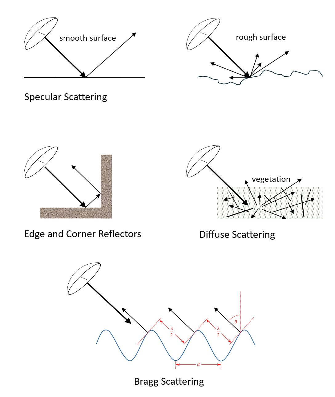
1. Specular (Mirror-like) Scattering
When the radar wavelength is much larger than surface roughness features, the surface appears smooth and acts like a mirror, reflecting energy away from the sensor (Woodhouse 2017). This produces very low backscatter. Calm water bodies, paved roads, and recently tilled agricultural fields often exhibit specular scattering, appearing dark in radar images.
The Rayleigh roughness criterion defines surface smoothness (Ulaby and Long 2013):
\[h < \frac{\lambda}{32 \cos \theta_i}\]
where h is RMS surface height variation, λ is wavelength, and θi is incidence angle. Surfaces satisfying this criterion produce predominantly specular scattering.
2. Diffuse (Rough Surface) Scattering
When surface roughness features approach or exceed the radar wavelength, scattering becomes diffuse, distributing energy in multiple directions including back toward the sensor (Henderson and Lewis 1998). This creates moderate to high backscatter depending on roughness magnitude and orientation. Natural surfaces like soil, rock, and vegetation typically produce diffuse scattering.
For moderate roughness, the backscattering coefficient increases with surface roughness until saturation occurs when roughness greatly exceeds the wavelength (Fung 1994).
3. Double-Bounce (Dihedral) Scattering
Corner reflector geometry—created by perpendicular or near-perpendicular surfaces—produces extremely strong backscatter through double-bounce reflection (Figure 7 panel c). The radar pulse reflects from one surface onto another, then back toward the sensor, creating backscatter intensities that can be 10-20 dB higher than rough surface scattering (Henderson and Lewis 1998).
Double-bounce mechanisms are characteristic of: - Urban areas: Building walls and ground create vertical-horizontal dihedrals - Flooded vegetation: Water surface and vertical stems create strong double-bounce returns - Tree trunks and ground: In forests, trunk-ground interaction produces significant double-bounce contribution
The mathematical description of double-bounce scattering from dihedrals depends on polarization, but generally produces strong HH and VV returns with distinct phase relationships (Ulaby and Long 2013).
4. Volume Scattering
Complex three-dimensional structures—particularly vegetation canopies—produce volume scattering through multiple interactions within the scattering volume (Figure 7 panel d). Radar energy penetrates into the canopy, scatters from leaves, branches, and stems at multiple levels, with some energy reaching the ground and scattering back through the canopy (Kasischke et al. 2019).
Volume scattering is characterized by: - Depolarization: Multiple scattering randomizes polarization, producing strong cross-polarized returns (HV, VH) - Wavelength dependence: Longer wavelengths penetrate deeper, interacting with larger structural elements - Complex phase behavior: Multiple path lengths create phase diversity that reduces interferometric coherence
For forests, volume scattering dominates at HV polarization and increases with forest density and biomass (Le Toan et al. 2011). The depth of penetration—and thus which structural elements contribute most to backscatter—depends critically on wavelength, as discussed in the following section.
5. Bragg Scattering
When surfaces exhibit periodic structure (waves, sand ripples, furrows), and the periodicity matches the radar wavelength, constructive interference produces enhanced backscatter through Bragg scattering (Woodhouse 2017). The Bragg condition is:
\[\lambda = 2 d \sin \theta_i\]
where d is the surface periodicity spacing. This mechanism is particularly important for ocean wave imaging, where capillary waves and gravity waves satisfying the Bragg condition create strong returns that enable measurement of wave spectra and surface wind fields (Moreira et al. 2013).
5.3 Permittivity and Moisture Effects
Beyond geometry, the dielectric constant (or relative permittivity, εr) profoundly affects radar backscatter. The dielectric constant determines how much electromagnetic energy is reflected versus transmitted at boundaries (Ulaby and Long 2013):
\[\Gamma = \frac{\sqrt{\varepsilon_{r1}} - \sqrt{\varepsilon_{r2}}}{\sqrt{\varepsilon_{r1}} + \sqrt{\varepsilon_{r2}}}\]
where Γ is the reflection coefficient and εr1, εr2 are the dielectric constants of the two media.
Crucially, liquid water has a very high dielectric constant (εr ≈ 80 at microwave frequencies) compared to dry soil (εr ≈ 3-5), dry vegetation (εr ≈ 2-10), and ice (εr ≈ 3) (Ulaby and Long 2013). This means:
- Wet surfaces reflect strongly (high Γ) → high backscatter
- Dry surfaces reflect weakly (low Γ) → lower backscatter
- Moisture content changes cause substantial backscatter variations
This sensitivity to moisture is both an opportunity—enabling soil moisture mapping and vegetation water content estimation—and a challenge, as moisture variations can mask structural changes of interest (Wigneron et al. 2017).
Figure 6 demonstrates these combined effects: the water body’s backscatter changes dramatically with wind conditions (flat water is specular and dark; rough water produces diffuse scattering and appears brighter), buildings show corner reflections or shadows depending on orientation, and terrain slope affects the local incidence angle and thus scattering mechanism.
Understanding these scattering mechanisms is essential for interpreting radar signatures of forests and other land cover types, where multiple mechanisms occur simultaneously and their relative contributions change with sensor parameters and environmental conditions.
6 Wavelength-Dependent Interactions
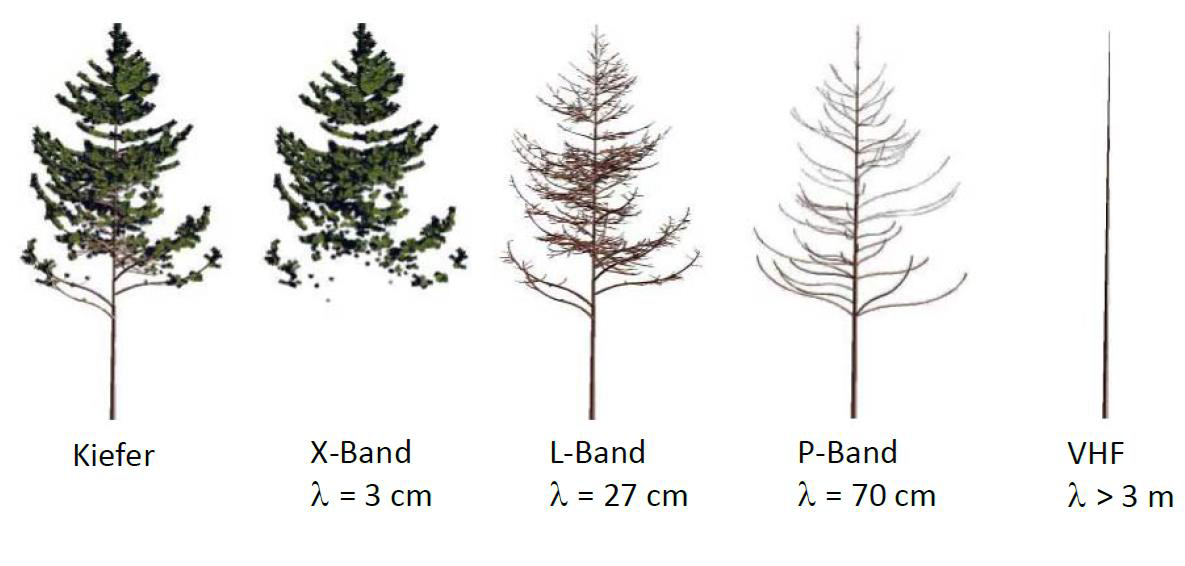
One of the most fundamental principles governing radar remote sensing of vegetation is that scattering occurs primarily from objects whose size is comparable to or larger than the radar wavelength (Ulaby and Long 2013). This wavelength dependence creates dramatic differences in how various radar frequencies interact with forest canopies, determining which structural elements contribute most to the observed backscatter.
Figure 8 illustrates this principle by showing a single tree structure as “seen” by different radar wavelengths. The progression from left to right—X-band (λ = 3 cm) through L-band (λ = 27 cm) to P-band (λ = 70 cm) and VHF (λ > 3 m)—reveals how longer wavelengths progressively see through smaller structural elements to interact with larger components deeper in the canopy.
6.1 Standard Radar Frequency Bands
Radar systems are conventionally designated by letter bands that originated in military secrecy during World War II but now serve as standard nomenclature (Woodhouse 2017). Figure 9 shows the most important bands for Earth observation:
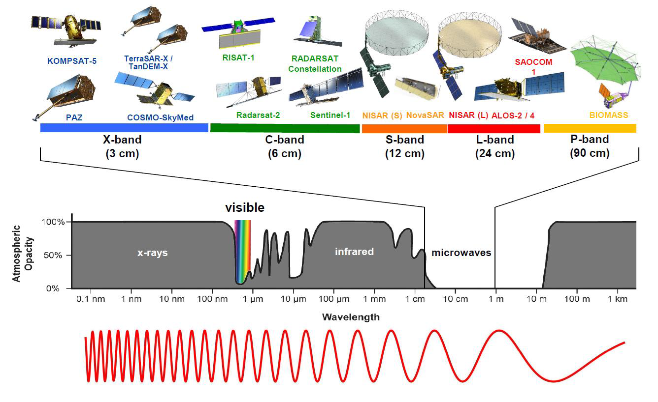
The key bands for vegetation remote sensing are (Kasischke et al. 2019):
X-band (~3 cm, ~10 GHz): Interacts with leaves, needles, and very small branches. Limited canopy penetration. Used for high-resolution urban and ice mapping. Systems include TerraSAR-X, TanDEM-X, COSMO-SkyMed.
C-band (~6 cm, ~5 GHz): Interacts with leaves, small branches, and crop structure. Moderate canopy penetration. Optimal for agricultural monitoring and widely used operationally. Systems include Sentinel-1 (operational), Radarsat-2, and the retired ERS and Envisat.
S-band (~12 cm, ~3 GHz): Intermediate penetration, sensitive to medium branch structure. Less commonly used but planned for NISAR mission.
L-band (~24 cm, ~1.5 GHz): Penetrates through foliage to interact with larger branches and trunks. Sensitive to forest structure and biomass. Systems include ALOS PALSAR (retired), ALOS-2, SAOCOM, and the upcoming NISAR mission.
P-band (~70 cm, ~450 MHz): Deep penetration to ground level even in dense forests. Interacts primarily with large branches and trunks. Optimal for biomass estimation. ESA’s BIOMASS mission (launch planned) will be the first spaceborne P-band SAR.
6.2 Penetration Depth and Biomass Sensitivity
The penetration depth—the distance that radar energy travels into vegetation before being completely scattered or absorbed—increases with wavelength according to approximately (Le Toan et al. 2011):
\[\delta \propto \frac{\lambda}{k_e}\]
where ke is the extinction coefficient of the vegetation, which depends on biomass density, moisture content, and structural complexity. Empirically, penetration depth scales roughly linearly with wavelength for forest canopies.
This wavelength-dependent penetration creates characteristic sensitivities to forest biomass:
Short wavelengths (X, C-band) saturate at low biomass (~20-60 Mg/ha) because scattering occurs entirely in the upper canopy; once this layer is dense, additional biomass below contributes minimally to backscatter (Kasischke et al. 2019).
Medium wavelengths (L-band) penetrate deeper and remain sensitive to higher biomass (~100-150 Mg/ha) by interacting with larger structural elements throughout the canopy (Mitchard et al. 2009).
Long wavelengths (P-band) penetrate to the ground even in dense tropical forests and maintain sensitivity to biomass approaching 500 Mg/ha, making them essential for global carbon monitoring in high-biomass ecosystems (Le Toan et al. 2011).
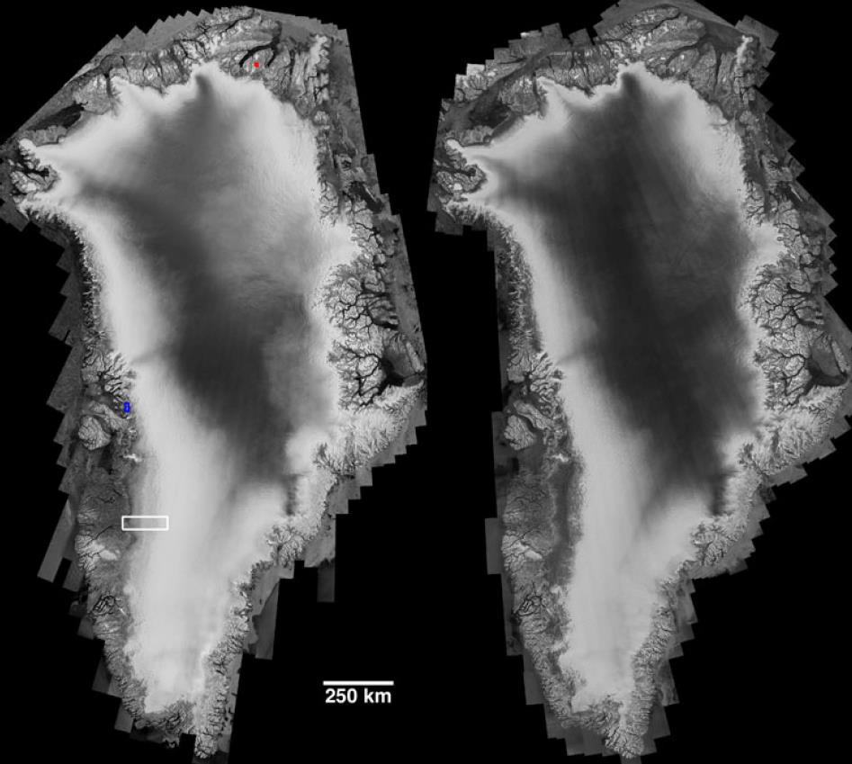
Figure 10 shows this principle with actual satellite data: RADARSAT (C-band) and ALOS PALSAR (L-band) images of the same area in Greenland reveal strikingly different surface expressions due to their different interaction depths (Joughin et al. 2016).
6.3 Implications for Forest Monitoring
The wavelength-dependent nature of radar-vegetation interaction has profound implications for application selection:
For biomass estimation: L-band or P-band are essential in moderate to high biomass forests, as shorter wavelengths saturate too quickly. Global biomass mapping requires spaceborne L-band or P-band systems (Saatchi et al. 2011).
For deforestation detection: C-band systems like Sentinel-1 are effective because clearcutting removes the scattering canopy, creating large backscatter changes even at wavelengths that see only upper canopy in intact forest (Bouvet et al. 2018).
For crop monitoring: C-band provides optimal sensitivity to crop structure and soil moisture throughout the growing season without excessive penetration (McNairn and Shang 2016).
For forest structure: L-band provides good sensitivity to canopy structure parameters including height, gap fraction, and vertical complexity (Treuhaft et al. 2010).
For subsurface imaging: P-band and VHF enable detection of subsurface features, including archaeological remains beneath forest canopy and ice structure beneath dry snow (Moreira et al. 2013).
7 Polarization: A Multi-Dimensional View
Beyond wavelength, polarization—the orientation of the electromagnetic field—provides an additional dimension for characterizing surface and volume scattering properties. Polarimetric radar systems transmit and receive both horizontally (H) and vertically (V) polarized radiation, enabling measurement of how surfaces and volumes transform polarization through scattering (S. Cloude 2009).
7.1 Polarization Fundamentals
An electromagnetic wave’s polarization describes the orientation of its electric field vector. For radar remote sensing, we conventionally define polarization relative to the plane containing the radar line of sight and the local vertical (Woodhouse 2017):
- Horizontal (H): Electric field perpendicular to this plane
- Vertical (V): Electric field parallel to this plane
A radar system can transmit at one polarization and receive at the same or different polarization, creating four possible combinations called polarization channels (Lee and Pottier 2009):
- HH: Transmit horizontal, receive horizontal (co-polarized)
- VV: Transmit vertical, receive vertical (co-polarized)
- HV: Transmit horizontal, receive vertical (cross-polarized)
- VH: Transmit vertical, receive horizontal (cross-polarized)
Due to reciprocity (for most natural surfaces), HV = VH, so only three independent measurements are available (S. Cloude 2009).
7.2 Polarimetric Modes
Different radar systems offer various polarimetric capabilities:
Single polarization: Transmits and receives only one polarization (HH or VV). Simplest mode, used for routine monitoring. Example: Sentinel-1 in Extra Wide Swath mode (Torres et al. 2012).
Dual polarization: Transmits one polarization and receives both (VV+VH or HH+HV). Provides sensitivity to depolarization from volume scattering. Example: Sentinel-1 in Interferometric Wide Swath mode (Torres et al. 2012), Envisat.
Alternating polarization:Sswitches between tranmitting H and V and receiving the same polarization (or often both). Example: Envisat.
Compact polarimetry: Transmits circular polarization and receives H and V, providing partial polarimetric information with reduced data volume (Raney 2007). Example: RADARSAT-2.
Quad polarization (full polarimetry): Transmits both H and V, receives all four combinations, capturing the complete scattering matrix. Provides maximum information but at reduced spatial coverage. Example: RADARSAT-2, ALOS-2 in polarimetric mode (S. Cloude 2009).
7.3 Scattering Behavior by Polarization
Different scattering mechanisms produce characteristic polarimetric signatures (Figure 11):
Surface scattering (smooth or moderately rough surfaces): - Strong co-polarized returns (HH, VV) - Weak cross-polarized returns (HV ≈ 0) - VV typically stronger than HH at moderate incidence angles (Ulaby and Long 2013)
Double-bounce scattering (corner reflectors, ground-trunk interaction): - Very strong HH and VV - Minimal cross-polarization - The relative strength of HH vs VV depends on surface properties (Henderson and Lewis 1998)
Volume scattering (vegetation, rough surfaces, snow): - Strong cross-polarized returns (HV, VH) - Depolarization caused by multiple scattering events randomizing polarization - HV is diagnostic of volume scattering (Kasischke et al. 2019)
The table in Table 1 summarizes the relative scattering strength by mechanism and polarization:
| Scattering Mechanism | HH/VV | HV/VH | Diagnostic Feature |
|---|---|---|---|
| Rough Surface | High | Low | |SVV| > |SHH| > |SHV| |
| Double Bounce | Very High | Very Low | |SHH| > |SVV| > |SHV| |
| Volume Scattering | Moderate | High | Main source of |SHV| |
7.4 Forest Applications of Polarimetry
Polarimetric data enable several important applications in forest remote sensing:
1. Forest/Non-Forest Classification
The high HV backscatter from volume scattering in forests contrasts sharply with the low HV from bare soil or water, enabling robust forest mapping even when HH or VV responses are ambiguous (Santoro et al. 2011).
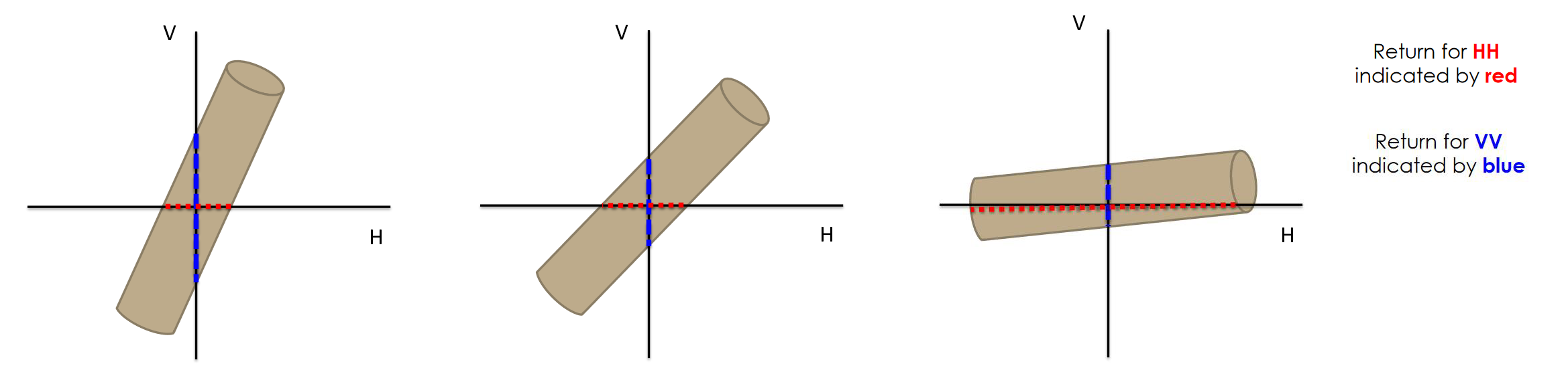
2. Forest Type Discrimination
Different forest types exhibit distinct polarimetric signatures: coniferous forests with vertical trunk structure show enhanced VV, deciduous forests with more horizontal branch orientation favor HH, and forest structure metrics like crown density affect depolarization strength (Lee and Pottier 2009).
3. Biomass Estimation Enhancement
Combining multiple polarizations improves biomass estimation by capturing both surface (HH, VV) and volume (HV) scattering components. Multi-polarization approaches extend the range of biomass sensitivity compared to single-polarization methods (Robinson et al. 2013).
4. Inundation Mapping in Forests
Flooded forests produce distinctive polarimetric signatures: strong HH/VV from double-bounce between water and trunks, combined with moderate HV from remaining canopy volume scattering. This combination allows detection of flooding beneath canopy cover (Henderson and Lewis 2008).
7.5 Polarimetric Decompositions
Advanced polarimetric analysis employs target decomposition methods that mathematically separate the measured backscatter into contributions from different scattering mechanisms (S. R. Cloude and Pottier 1997). Figure 12 shows various decomposition results applied to the same scene.
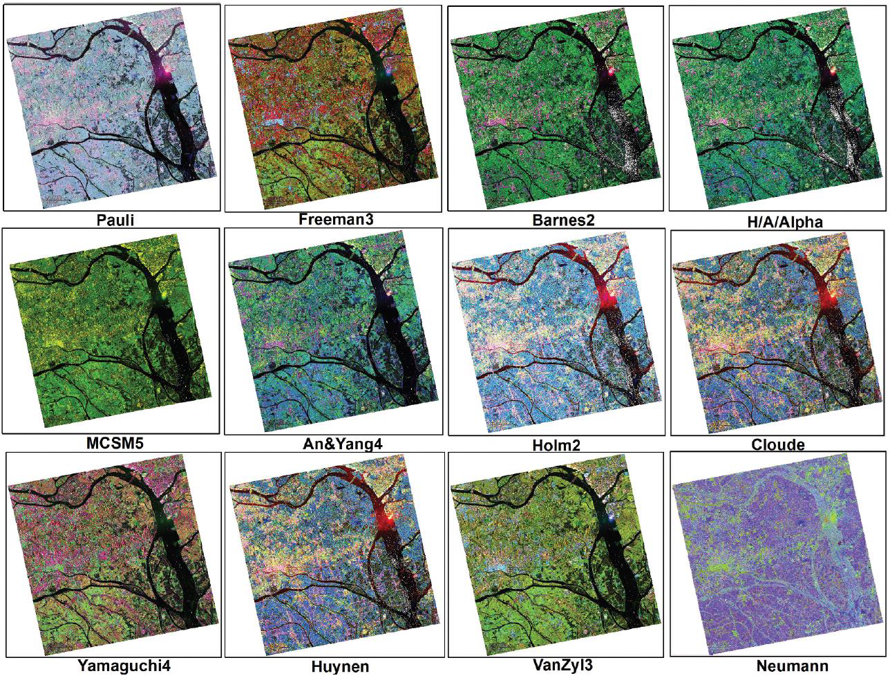
Common decompositions include:
- Pauli decomposition: Separates single-bounce, double-bounce, and volume scattering (Lee and Pottier 2009)
- Freeman-Durden decomposition: Models scattering as combination of surface, double-bounce, and volume components (Freeman and Durden 1998)
- Cloude-Pottier (H/A/α) decomposition: Uses entropy, anisotropy, and alpha angle to characterize scattering randomness and mechanism (S. R. Cloude and Pottier 1997)
- Yamaguchi decomposition: Extends Freeman-Durden with helix scattering term for complex oriented volumes (Yamaguchi et al. 2011)
These decompositions transform polarimetric data into interpretable scattering parameters, enhancing classification accuracy and providing physical insight into surface and volume properties (Lee and Pottier 2009).
8 Geometric Distortions in Radar Imaging
The side-looking geometry of radar systems, combined with the range-based measurement principle, creates characteristic geometric distortions that profoundly affect radar image geometry and require careful correction for quantitative analysis (Henderson and Lewis 1998). Unlike optical images where each pixel represents a fixed ground area, radar pixel spacing in range depends on local surface topography and viewing geometry.
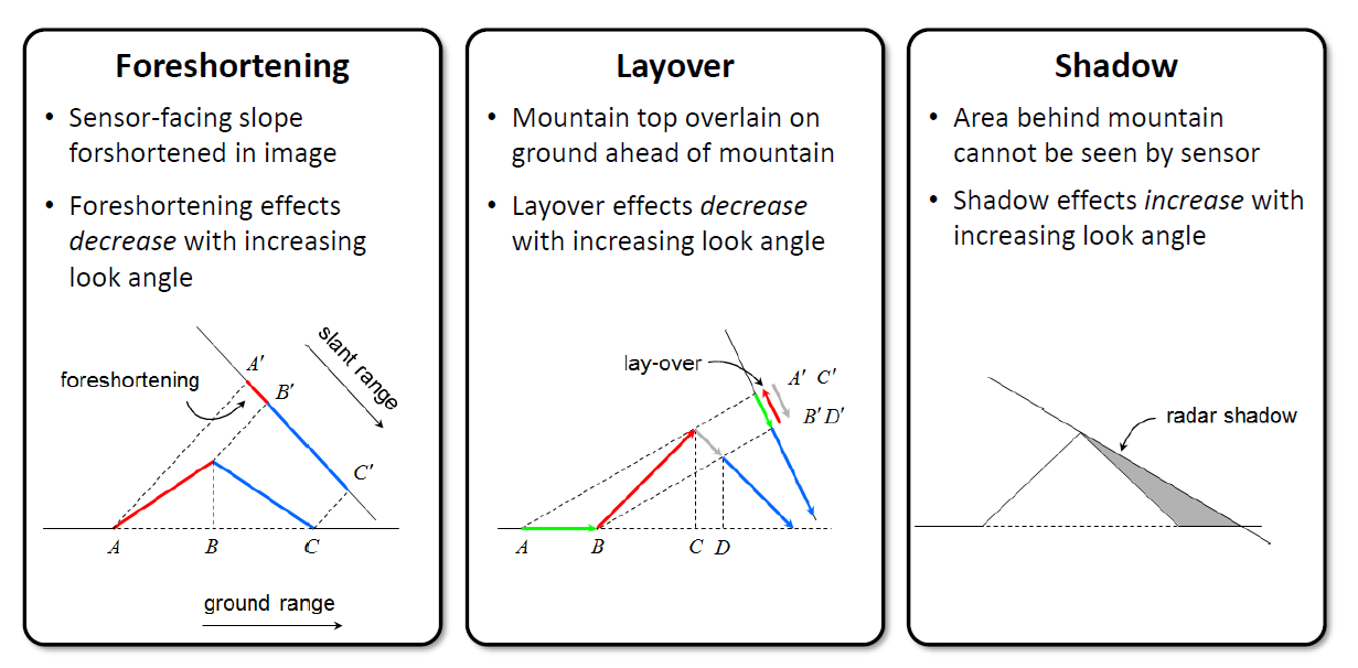
Three primary distortion types affect radar imagery: foreshortening, layover, and shadow. Understanding these effects is essential for radar image interpretation and for determining optimal imaging geometry for specific applications.
8.1 Foreshortening
Foreshortening occurs when terrain slopes toward the radar, causing the slant range distance between the slope base and crest to be compressed relative to the true ground distance (Figure 13 left panel). The effect is analogous to viewing a hillside from an oblique angle: features on the slope appear compressed in the viewing direction (Woodhouse 2017).
Mathematically, the compression factor for a uniform slope is (Henderson and Lewis 1998):
\[CF = \frac{R_{slant}}{R_{ground}} = \frac{\sin(\theta_i - \alpha)}{\sin(\theta_i)}\]
where θi is the radar incidence angle and α is the terrain slope angle (positive when sloping toward the radar).
Consequences of foreshortening: - Bright returns: Compressed terrain results in energy returned from a larger actual area concentrated into fewer image pixels, increasing pixel brightness - Distorted geometry: Distances and areas are incorrectly represented, affecting measurements - Reduced texture: Surface detail is compressed, potentially limiting interpretation
Foreshortening effects decrease with increasing look angle (more oblique views), as the angular difference between radar look angle and slope angle increases (Woodhouse 2017).
8.2 Layover
When terrain slope exceeds the radar depression angle, layover occurs: the top of the slope is closer to the radar in slant range than the base, causing these features to be imaged in reversed order (Figure 13 center panel). This geometric inversion is unique to radar and has no optical equivalent (Henderson and Lewis 1998).
The layover condition is met when (Woodhouse 2017):
\[\alpha > \theta_i\]
where α is terrain slope and θi is incidence angle.
Characteristics of layover: - Complete geometric reversal: Features at the slope top appear in front of (closer in range than) features at the base - Superposition: Signals from multiple elevations overlap in a single image location, mixing returns from different surface elements - Very bright returns: Multiple scattering surfaces contribute to the same pixels - Interpretation difficulty: Layover regions are essentially uninterpretable; features cannot be reliably identified
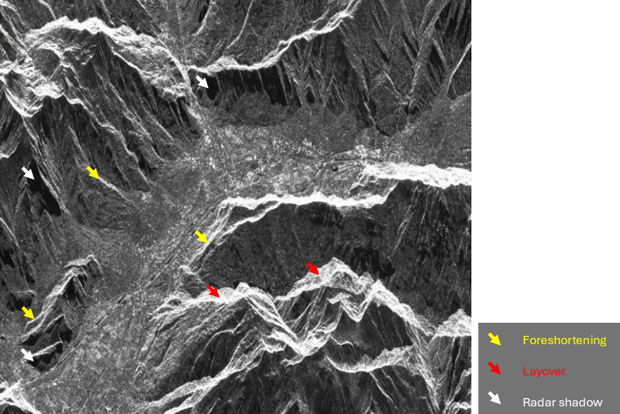
?@fig-mountain-distortions shows a dramatic real-world example: mountains in Alaska imaged by SAR exhibit severe foreshortening on the radar-facing slopes (very bright, compressed features) and shadow on the far slopes (no signal, black areas).
Layover increases with decreasing look angle (steeper views), as the probability that terrain slope exceeds radar incidence angle increases. Very steep look angles can cause layover even on moderate slopes.
8.3 Radar Shadow
Radar shadow occurs when terrain blocks the radar beam from illuminating areas behind topographic obstacles (Figure 13 right panel). Unlike optical shadows (caused by blocked sunlight), radar shadows result from blocked radar illumination from the specific side-looking viewing geometry (Henderson and Lewis 1998).
Shadow occurs when (Woodhouse 2017):
\[\alpha_{far} < -\theta_i\]
where αfar is the slope angle on the far side of a topographic feature (negative for slopes facing away from the radar).
Characteristics of radar shadow: - No signal return: Shadowed areas receive no radar illumination, resulting in zero or noise-level backscatter (appear black) - Complete information loss: No surface information can be retrieved from shadowed pixels - Sharp boundaries: Shadow edges are geometrically well-defined by terrain and viewing geometry - Can be useful: Shadow provides strong topographic information and can enhance 3D perception of terrain relief
Shadow extent increases with decreasing look angle (steeper views) and increases with increasing terrain relief. Calculating shadow extent requires detailed topographic information (DEM) and precise orbit geometry (Small 2011).
8.4 Mitigating Geometric Distortions
Several strategies minimize or correct geometric distortions (Henderson and Lewis 1998; Small 2011):
1. Imaging Geometry Selection
- Moderate incidence angles (30-40°) balance foreshortening (worse at steep angles), layover (worse at steep angles), and shadow (worse at shallow angles)
- Multiple viewing geometries: Ascending and descending pass combinations image opposite slope faces, ensuring one geometry avoids layover/shadow for each feature
- Right-side and left-side looking: Some satellites can point the radar beam to either side, providing geometric diversity
2. Terrain Correction
Radiometric terrain correction compensates for local incidence angle effects caused by topography, normalizing backscatter to a reference geometry (Small 2011). This requires: - High-quality Digital Elevation Model (DEM) - Precise orbit and sensor geometry information - Radiometric calibration
The correction adjusts pixel values based on local geometry:
\[\sigma°_{corrected} = \sigma°_{measured} \times \frac{\sin \theta_{ref}}{\sin \theta_{local}}\]
where θlocal is the local incidence angle accounting for topography, and θref is the reference incidence angle (Ulander 1996).
3. Geocoding and Orthorectification
Geometric terrain correction (orthorectification) transforms radar images from slant range geometry to map coordinates, correcting foreshortening and compensating for terrain elevation (Small 2011). This process: - Requires a DEM to determine true ground positions - Corrects pixel spacing for terrain slope - Enables integration with GIS data and other sensors - Cannot recover information from layover or shadow, which remain as distortions
4. Masking Unreliable Areas
For quantitative analysis, pixels affected by severe layover or shadow are typically masked and excluded from analysis, as their values do not reliably represent surface properties (Santoro et al. 2011).
In forest applications, geometric distortions are less severe than in mountainous terrain, as forest canopy topography is gentler. However, even moderate slopes can create significant foreshortening effects that must be corrected for accurate biomass estimation or change detection (Cartus, Santoro, and Kellndorfer 2012).
9 Speckle: Coherent Noise in Radar Images
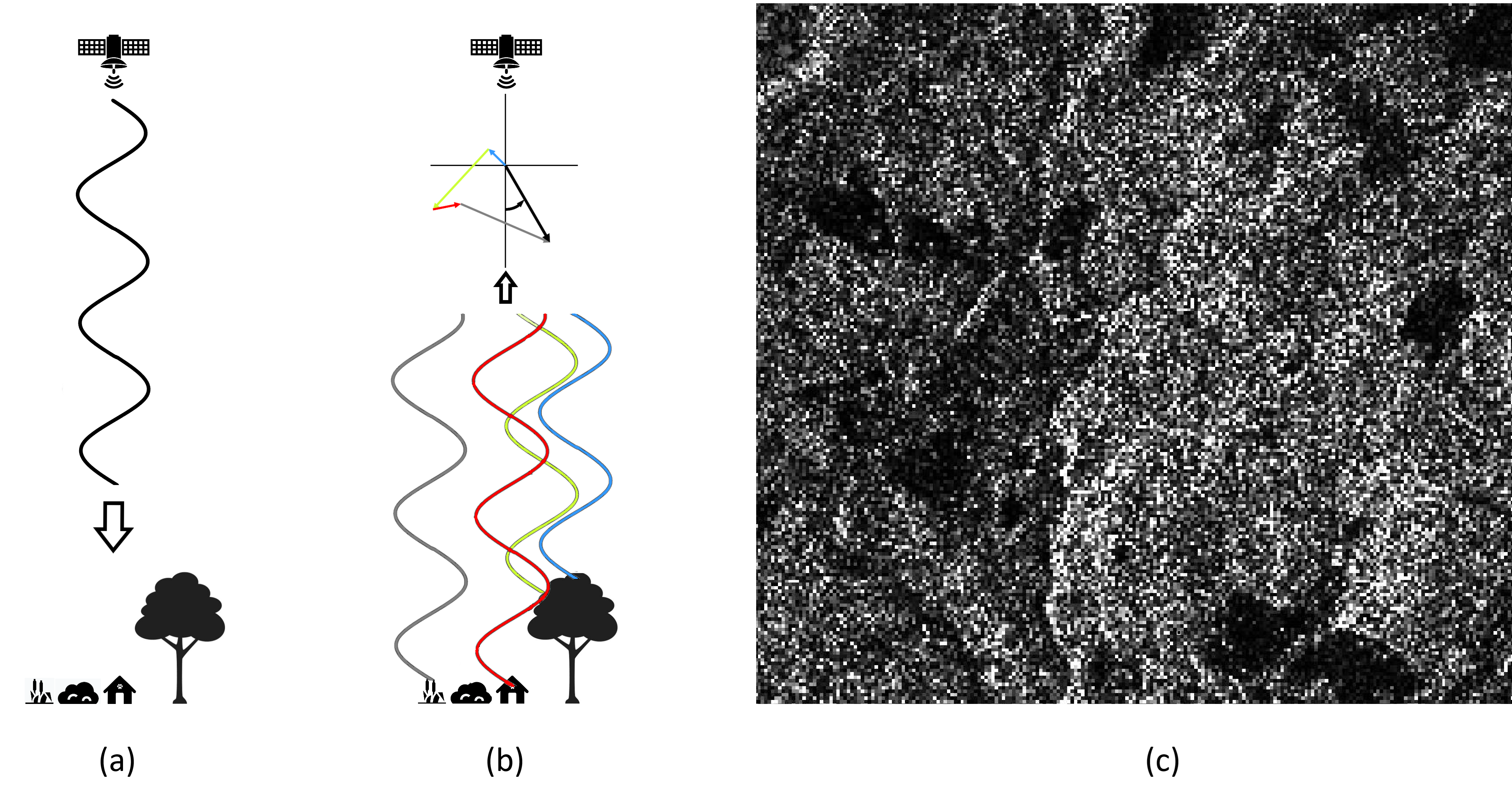
Unlike optical images where pixel values represent incoherent addition of reflected energy from multiple scatterers within the resolution cell, radar images are formed from coherent summation of returns from all scatterers, preserving phase relationships (Goodman 1976). This coherent imaging process creates speckle—a granular noise pattern that is not sensor noise but rather an intrinsic consequence of coherent detection from random scatterers within a resolution cell.
Figure 15 illustrates the physical origin of speckle. When multiple scatterers within a resolution cell reflect the radar signal, each reflection returns with a specific amplitude (determined by the scatterer’s radar cross section) and phase (determined by the distance traveled). Because radar preserves phase information, these individual returns coherently interfere—adding constructively where phases align and destructively where phases oppose (Lee and Pottier 2009).
9.1 Speckle Statistics
For a resolution cell containing many independent scatterers with random phases, the resulting intensity follows specific probability distributions (Goodman 1976; Lee 1981):
Single-look intensity: The backscatter intensity I from one image (one “look”) follows a negative exponential (gamma) distribution:
\[p(I) = \frac{1}{\langle I \rangle} \exp\left(-\frac{I}{\langle I \rangle}\right)\]
where ⟨I⟩ is the mean intensity. This distribution has standard deviation equal to the mean, creating a signal-to-noise ratio (SNR) of 1 (0 dB) (Lee and Pottier 2009).
Multi-look intensity: Averaging N independent looks reduces speckle. The multi-look intensity follows a gamma distribution with shape parameter N:
\[p(I_N) = \frac{N^N}{\Gamma(N)\langle I \rangle^N} I^{N-1} \exp\left(-\frac{NI}{\langle I \rangle}\right)\]
The resulting SNR improves to \(\sqrt{N}\) (Lee 1981), making multi-looking the fundamental speckle reduction technique.
9.2 Visual Impact
Figure 15 (c) shows the characteristic appearance of speckle: a scene that should appear uniform (same surface type, in this case forest) exhibits random pixel-to-pixel intensity variation. This “salt and pepper” texture is present throughout radar images, obscuring fine spatial detail and complicating image interpretation and classification (Lee and Pottier 2009).
Key characteristics of speckle (Goodman 1976):
- Multiplicative: Speckle variance increases proportionally with signal level (unlike additive sensor noise)
- Spatially correlated: Adjacent pixels show some correlation at scales comparable to the resolution
- Fully developed: In single-look images, the speckle standard deviation equals the mean
- Not random noise: Each speckle pattern is deterministic for a given scene and viewing geometry; repeated observations from identical geometry would produce identical speckle (Zebker and Villasenor 1992)
9.3 Speckle Reduction Strategies
Several approaches mitigate speckle’s impact on radar image analysis (Lee and Pottier 2009; Lee 1981):
1. Multi-looking (Spatial Averaging)
Dividing the synthetic aperture into sub-apertures creates multiple independent images (“looks”) of the same scene. Averaging these looks reduces speckle at the cost of degraded spatial resolution (Oliver and Quegan 1991):
\[\text{Speckle reduction} = \sqrt{N_{looks}}\] \[\text{Resolution degradation} = \sqrt{N_{looks}}\]
Typical operational SAR products use 3-5 looks in range and azimuth, trading ~3-5 dB speckle reduction for similar resolution loss (Torres et al. 2012).
2. Spatial Filtering
Adaptive filters apply local averaging weighted by spatial statistics, attempting to smooth speckle while preserving edges and features (Lee 1981; Frost et al. 1982). Common filters include:
- Lee filter: Adapts averaging based on local coefficient of variation (Lee 1981)
- Frost filter: Uses exponential kernel weighted by local statistics (Frost et al. 1982)
- Gamma MAP filter: Maximum a posteriori estimation assuming gamma distribution (Lopes et al. 1990)
These filters improve speckle suppression compared to simple averaging but still trade spatial resolution for speckle reduction.
3. Multi-temporal Averaging
Averaging images from different dates reduces speckle if scene properties remain stable, as speckle patterns differ between acquisitions (Quegan and Yu 2001):
\[\text{Speckle reduction} = \sqrt{N_{dates}}\]
This approach is particularly effective for forest monitoring where temporal change is slow, though care must be taken not to average over genuine changes of interest (Santoro et al. 2011).
4. Transform-Domain Filtering
Sophisticated techniques decompose images into spatial or frequency domains, apply selective filtering, and reconstruct (Deledalle, Denis, and Tupin 2015). These include:
- Wavelet-based methods: Exploit multi-scale speckle characteristics (Argenti et al. 2013)
- Non-local means: Leverage image self-similarity for averaging (Deledalle, Denis, and Tupin 2015)
- Total variation methods: Preserve edges while smoothing homogeneous areas (Denis et al. 2006)
These advanced methods achieve better feature preservation than traditional filters but at higher computational cost (Argenti et al. 2013).
9.4 Speckle Tracking and Offset Tracking
Interestingly, speckle that complicates radiometric analysis can be exploited for motion detection. Speckle tracking (or offset tracking) measures displacement by correlating speckle patterns between repeat-pass images (Strozzi et al. 2002). Because each speckle pattern is unique and deterministic, surface displacement shifts the entire pattern, enabling measurement of:
- Glacier flow: Surface velocity fields from pattern displacement (Rignot et al. 1995)
- Landslide movement: Slow-moving slope failures detected by pattern shift (Singleton et al. 2014)
- Earthquake deformation: Co-seismic displacement fields exceeding interferometric limits (Michel, Avouac, and Taboury 1999)
This technique works even when interferometric coherence is lost, though with lower precision (~1/10 pixel) than interferometry (~1/100 wave) (Strozzi et al. 2002).
9.5 Implications for Forest Monitoring
In forest remote sensing, speckle affects applications differently (Kasischke et al. 2019):
- Biomass estimation: Speckle introduces estimation uncertainty; multi-looking and filtering are essential for reducing variance in biomass predictions (Santoro et al. 2021)
- Change detection: Temporal filtering reduces false alarms from speckle-induced differences, but thresholds must account for speckle statistics (Reiche et al. 2015)
- Classification: Texture measures derived from speckle patterns can improve forest type discrimination (Kumar et al. 2014), turning a challenge into a feature
Understanding speckle as coherent interference rather than random noise is fundamental to developing effective processing strategies and correctly interpreting radar statistics in forest and other land cover applications.
10 Phase Information: Interferometry and Beyond
Unlike optical and infrared sensors that detect only intensity (brightness), radar systems measure both the amplitude and phase of the returned signal (Bamler and Hartl 1998). While amplitude corresponds to backscatter intensity and relates to surface roughness and dielectric properties, phase carries information about the distance traveled by the radar signal. This phase information, preserved through coherent detection, enables a powerful set of techniques collectively known as radar interferometry that can measure surface topography, detect subtle surface displacements, and characterize vegetation structure with extraordinary precision (P. A. Rosen et al. 2000).
10.1 Phase Fundamentals
For a radar signal with wavelength λ, the two-way path to a target at range R creates a phase shift (Bamler and Hartl 1998):
\[\phi = \frac{4\pi R}{\lambda}\]
The factor of 4π (rather than 2π) appears because the signal travels to the target and back, covering distance 2R. Any change in range—whether from topography, surface displacement, or atmospheric effects—creates a corresponding phase change (Hanssen 2001).
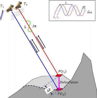
Figure 16 illustrates this concept. Two observations of the same point P at slightly different times (t₁ and t₂) show a change in range (ΔR) due to surface deformation. This range change produces a measurable phase difference:
\[\Delta \phi = \frac{4\pi \Delta R}{\lambda}\]
10.2 Interferometric SAR (InSAR)
Interferometric SAR creates an interferogram by multiplying one complex SAR image with the conjugate of another and extracting the phase difference (Bamler and Hartl 1998):
\[\phi_{int} = \arg(S_1 \cdot S_2^*)\]
where S₁ and S₂ are complex SAR images from two acquisitions. The resulting interferometric phase contains contributions from (Hanssen 2001):
\[\phi_{int} = \phi_{flat} + \phi_{topo} + \phi_{defo} + \phi_{atm} + \phi_{noise}\]
where: - φflat: Phase from flat-earth ellipsoid (depends on imaging geometry) - φtopo: Phase from surface topography - φdefo: Phase from surface displacement between acquisitions - φatm: Phase from atmospheric path delay differences - φnoise: Phase decorrelation and noise
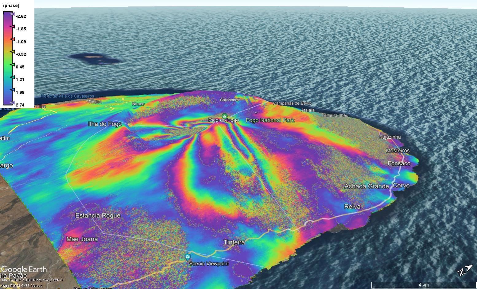
?@fig-interferogram shows a striking example: an interferogram of volcanic activity on Fogo Island, Cape Verde ?@fig-phase-volcano. The colored fringes—each cycle from blue through red to blue again represents one wavelength of phase change—map surface deformation with centimeter precision over the entire scene. The concentric fringe pattern centered on the volcano reveals inflation or deflation of the volcanic edifice.
10.3 Applications of InSAR
The sensitivity of phase to sub-wavelength changes enables diverse applications (P. A. Rosen et al. 2000; Hanssen 2001):
1. Topographic Mapping
Two SAR acquisitions from slightly different positions (creating a spatial baseline) produce interferometric phase that depends on topography. After removing flat-earth phase, the remaining phase directly relates to elevation (Zebker and Goldstein 1986):
\[h = \frac{\lambda R \sin \theta \Delta\phi_{topo}}{4\pi B_{\perp}}\]
where h is elevation, R is range, θ is look angle, and B⊥ is the perpendicular baseline between acquisition positions.
The TanDEM-X mission uses this principle with two satellites flying in close formation, achieving global topographic mapping with 12-meter horizonthal resolution and 2-meter relative vertical accuracy (Krieger et al. 2013).
2. Surface Displacement Measurement
Time-series of SAR acquisitions enable measurement of surface motion through differential interferometry (DInSAR), where topographic phase is subtracted using a DEM, leaving displacement phase (Massonnet et al. 1993):
\[\Delta R = \frac{\lambda \Delta\phi_{defo}}{4\pi}\]
Figure 18 shows a dramatic example: the 2003 Bam, Iran earthquake produced an interferogram with more than 50 fringes near the epicenter, indicating ~1.5 meters of surface displacement (Funning et al. 2005). The complexity of the fringe pattern reveals details of fault geometry and slip distribution.
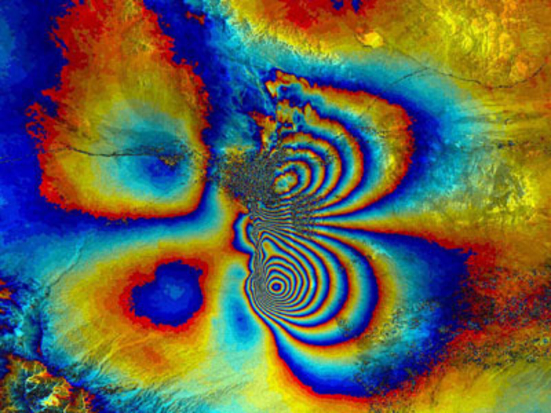
A key advantage of radar interferometry for earthquake monitoring is the ability to observe surface conditions both before and after seismic events. The interferogram reveals two distinct deformation centers connected by a linear feature—the surface expression of the fault rupture. When tectonic pressure causes the crust to fracture, one block of the Earth’s surface moves upward while the adjacent block subsides. The direction of vertical motion can be determined from the color sequence in the fringe pattern: areas where colors progress from red through yellow to green indicate uplift, while the reverse sequence (green through yellow to red) indicates subsidence. This bidirectional deformation pattern, combined with the spatial distribution of fringes, enables precise determination of the earthquake epicenter location and the geometry of the causative fault structure without requiring ground-based measurements.
Applications include: - Earthquake deformation: Co-seismic and post-seismic displacement fields (Massonnet et al. 1993) - Volcano monitoring: Magma inflation/deflation cycles (Massonnet, Briole, and Arnaud 1995) - Subsidence measurement: Groundwater extraction, mining, permafrost thaw (Galloway and Burbey 2011) - Glacier flow: Ice velocity through offset tracking and interferometry (Rignot et al. 1995) - Landslide monitoring: Slow-moving slope instabilities (Singleton et al. 2014)
3. Operational Ground Motion Services
The European Ground Motion Service provides systematic InSAR-derived displacement measurements across Europe, updating regularly and freely available (Dehls et al. 2019).
4. Forest Structure and Biomass
In vegetated areas, interferometric phase becomes more complex. The phase center—the elevation from which the effective scattering originates—depends on wavelength-dependent penetration depth (Treuhaft and Siqueira 1996):
- Short wavelengths (X, C-band): Phase center near canopy top
- Long wavelengths (L, P-band): Phase center within canopy, sensitive to vertical structure
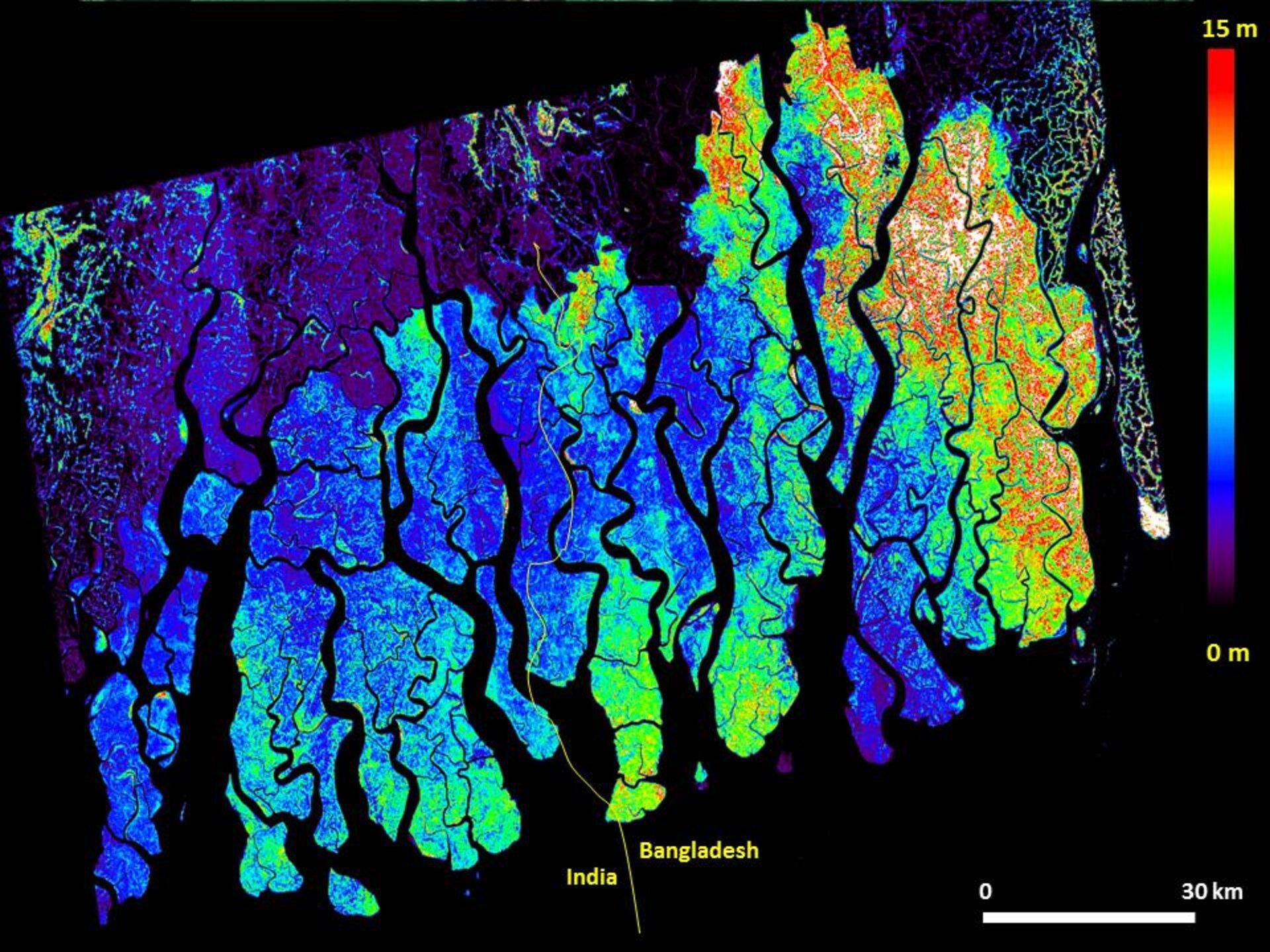
Polarimetric interferometry (PolInSAR) combines polarimetry and interferometry to separate ground and canopy contributions, enabling extraction of forest height, vertical profile, and biomass from the interferometric phase structure (S. R. Cloude and Papathanassiou 2003). ?@fig-polinsar-forest shows forest height derived from this technique for the Sundarbans mangrove forest.
5. Soil Moisture Estimation
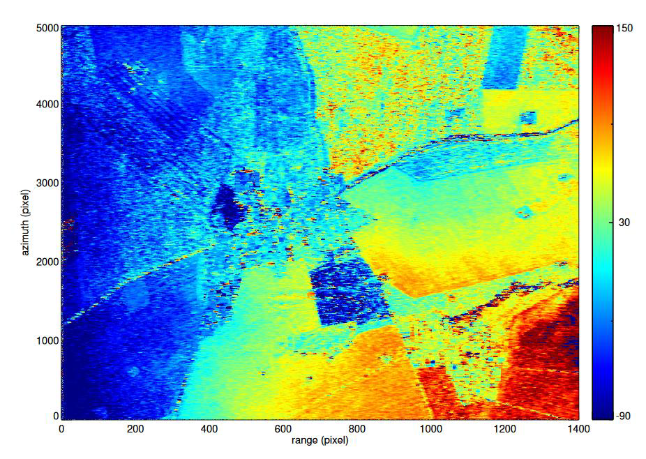
Changes in soil moisture alter the dielectric constant, changing penetration depth and thus phase. ?@fig-soil-moisture shows an interferogram sensitive to sub-surface moisture changes, where phase variations correlate with irrigation patterns and moisture gradients (De Zan et al. 2014).
10.4 Coherence and Decorrelation
Interferometry requires that the two SAR images maintain coherence—the speckle patterns must remain sufficiently similar that phase differences are meaningful (Zebker and Villasenor 1992). The interferometric coherence is defined as:
\[\gamma = \frac{|\langle S_1 S_2^* \rangle|}{\sqrt{\langle |S_1|^2 \rangle \langle |S_2|^2 \rangle}}\]
ranging from 0 (completely decorrelated, phase meaningless) to 1 (perfectly coherent, phase precise) (Bamler and Hartl 1998).
Decorrelation sources include: - Temporal decorrelation: Surface changes (vegetation growth, snow, moisture) between acquisitions (Zebker and Villasenor 1992) - Geometric decorrelation: Different viewing angles create different scattering paths (Bamler and Hartl 1998) - Volume decorrelation: In vegetation, scatterers distributed through depth create phase diversity (Treuhaft and Siqueira 1996) - Processing errors: Co-registration errors, phase unwrapping mistakes (Hanssen 2001)
For vegetation, temporal coherence decays rapidly (days to weeks at C-band) due to wind-induced motion, growth, and moisture changes (Wegmüller and Werner 1995). This limits repeat-pass interferometry over forests, though very short temporal baselines (1-day for Sentinel-1 over Europe) or longer wavelengths (L-band maintains coherence longer) mitigate this issue (Santoro et al. 2021).
10.5 Phase Unwrapping
Measured interferometric phase is wrapped into the range [-π, +π], creating 2π ambiguities (Ghiglia and Pritt 1998). Phase unwrapping resolves these ambiguities to recover the continuous phase field representing physical displacement or topography (Goldstein, Zebker, and Werner 1988). This challenging inverse problem requires:
- High coherence (phase quality)
- Sufficient spatial sampling (fringe density not exceeding Nyquist)
- Reliable algorithms to identify and integrate phase gradients correctly (C. W. Chen and Zebker 2001)
Unwrapping failures create errors that propagate through the phase field, potentially corrupting large image regions (Bamler and Hartl 1998). Quality-guided algorithms and statistical cost-flow approaches improve robustness (Goldstein, Zebker, and Werner 1988; C. W. Chen and Zebker 2001).
11 Future Radar Missions and Emerging Capabilities
The coming years will see a dramatic expansion in spaceborne radar capabilities, driven by missions specifically designed for vegetation monitoring, systematic change detection, and advanced interferometric techniques (Moreira et al. 2013). These next-generation systems will provide unprecedented temporal resolution, wavelength diversity, and measurement sophistication for forest and ecosystem applications.
11.1 Near-Term Operational Missions
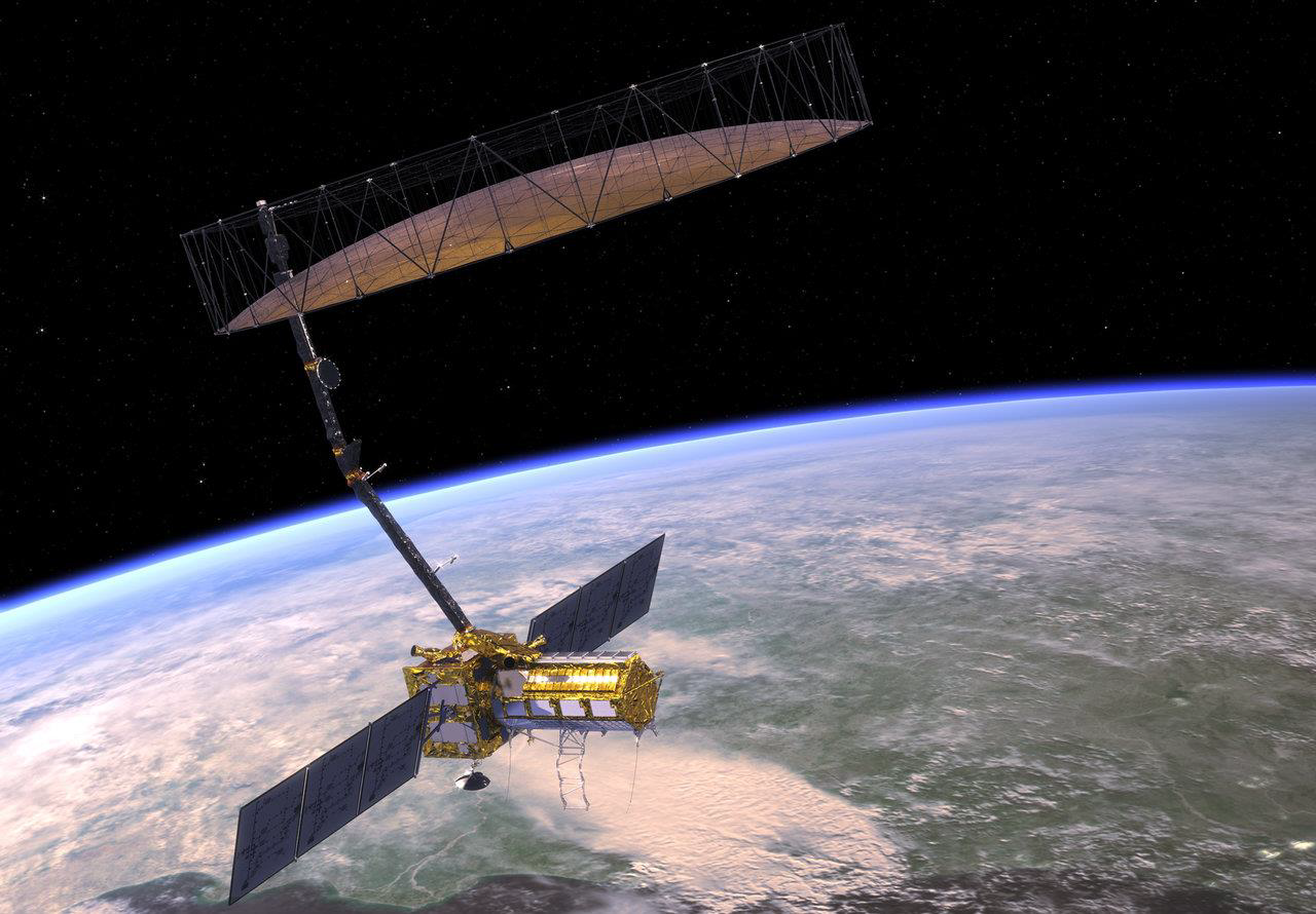
NISAR (NASA-ISRO SAR) (P. Rosen and Kumar 2017): Planned launch 2024, this joint NASA-ISRO mission will carry dual-frequency (L-band and S-band) SAR with 12-day repeat cycle and systematic global coverage. Key capabilities: - L-band (24 cm): Full polarimetry, 6-12 day repeat for biomass and forest structure - S-band (9 cm): Dual polarimetry for cropland and soil moisture monitoring - 240 km swath: Near-global coverage every 12 days enables change detection and time series analysis
Figure 21 shows the NISAR spacecraft with its large deployable antenna. NISAR’s systematic coverage and open data policy will revolutionize forest monitoring by providing consistent, high-quality L-band data globally (P. Rosen and Kumar 2017).
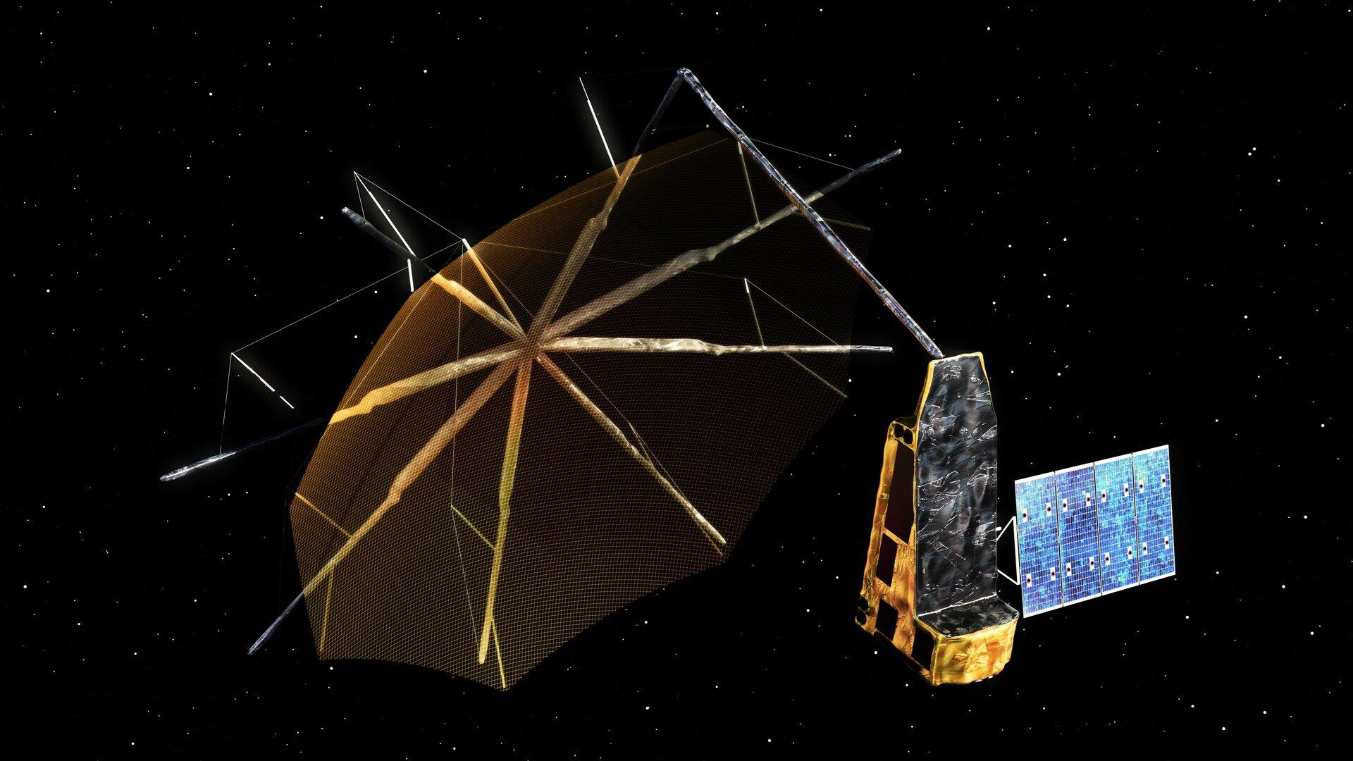
BIOMASS (ESA) (Le Toan et al. 2011): ESA’s first P-band spaceborne SAR, planned launch 2024, specifically designed for forest biomass estimation. Key innovations: - P-band (70 cm): Unprecedented penetration to ground even in dense tropical forests - Polarimetric and interferometric modes: Enable structure and height estimation - Tomographic capability: 3D imaging of forest vertical structure through repeated passes - Global forest mapping: Primary mission goal is global biomass estimation for carbon accounting
?@fig-biomass-mission shows the BIOMASS spacecraft with its distinctive large reflector antenna required for P-band operation. This mission will address the critical need for accurate tropical forest biomass estimates (Le Toan et al. 2011).
11.2 Advanced SAR Techniques for Forests
SAR Tomography (TomoSAR): By combining multiple SAR acquisitions from slightly different viewing angles (perpendicular baseline diversity), tomographic SAR reconstructs the three-dimensional distribution of scatterers (Reigber and Moreira 2000). Figure 23 illustrates the principle: multiple flight tracks create a synthetic aperture in the vertical dimension, enabling resolution of scatterer height.
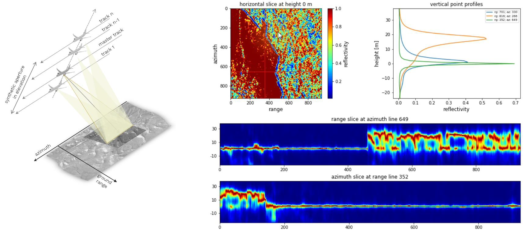
For forests, TomoSAR provides: - Vertical profile: Scattering intensity as function of height, related to biomass distribution (Tebaldini 2012) - Ground-canopy separation: Unambiguous identification of ground and vegetation returns (Tebaldini and Rocca 2010) - Understory detection: Sensitivity to understory vegetation beneath dominant canopy (Banda et al. 2016) - 3D structure metrics: Canopy complexity, layering, gaps (Minh et al. 2016)
Operational implementation requires: - Multiple baselines: At least 5-10 acquisitions with baseline diversity (Reigber and Moreira 2000) - High temporal coherence: Vegetation must remain stable across all acquisitions - Sophisticated processing: 3D focusing algorithms and parameter estimation (Fornaro, Serafino, and Soldovieri 2005)
Differential Tomography: Combining TomoSAR with temporal series enables measurement of 3D structure changes, potentially detecting selective logging or degradation that leaves the upper canopy intact but alters vertical profile (Tebaldini et al. 2020).
Polarimetric Tomography: Integrating polarimetry with tomography provides polarization-dependent vertical profiles, enabling discrimination of scattering mechanisms (ground, trunk, branch, leaf) at different heights (S. R. Cloude 2006).
See a dedicated chapter on TomoSAR in this e-learning materials.
11.3 Emerging Commercial Constellations
Beyond government missions, several commercial SAR constellations are emerging (Moreira et al. 2013):
Capella Space: First commercial SAR constellation providing sub-meter resolution X-band imagery on-demand.
ICEYE: Constellation of small X-band SAR satellites enabling rapid revisit and video-like monitoring.
While these commercial systems primarily target defense, maritime, and infrastructure monitoring, their high temporal resolution (potentially daily or better) could enable new forest monitoring applications, particularly for rapid deforestation detection or disaster response.
12 Physical and Semi-Empirical Models
Quantitative interpretation of radar signatures for forest parameters requires models linking backscatter to biophysical properties. These range from purely empirical statistical relationships to physical models solving Maxwell’s equations for electromagnetic scattering from complex forest structures (Ulaby and Long 2013).
12.1 The Water Cloud Model (WCM)
The simplest physically motivated model represents vegetation as a uniform cloud of water droplets above a soil surface (Attema and Ulaby 1978). The total backscatter is:
\[\sigma° = \sigma°_{veg} + \tau^2 \sigma°_{soil}\]
where σ°veg is vegetation volume scattering, σ°soil is soil surface scattering, and τ² is two-way transmissivity through the vegetation layer (Attema and Ulaby 1978).
The vegetation component is:
\[\sigma°_{veg} = A V_1 (1 - \tau^2) \cos \theta\]
and transmissivity is:
\[\tau^2 = \exp(-2 B V_2 \sec \theta)\]
where V₁ and V₂ are vegetation descriptors (often the same, e.g., LAI or biomass), A and B are fitting parameters, and θ is incidence angle (Bindlish and Barros 2000).
Despite its simplicity, WCM provides reasonable backscatter predictions for crops and grasslands and has been extended for forest applications by including stem and ground interaction terms (Kumar et al. 2016).
12.2 The Michigan Microwave Canopy Scattering Model (MIMICS)
MIMICS represents vegetation as discrete scatterers (leaves, branches, trunks) with specific sizes, orientations, and distributions, computing first-order scattering from each component plus ground interaction (Ulaby et al. 1990). The model:
- Discretizes canopy: Divides vegetation into layers and scatterer types
- Computes scattering: Uses scattering theory for cylinders (branches), discs (leaves), ground
- Sums contributions: Integrates over canopy depth accounting for attenuation
MIMICS requires detailed canopy structure inputs (height, density, orientation distributions) but provides polarimetric backscatter predictions without empirical calibration (Ulaby et al. 1990). This physical basis enables: - Sensitivity analysis: Determining which parameters affect backscatter most - Inversion: Retrieving canopy parameters from observed backscatter - Mission planning: Simulating expected performance of new sensors
12.3 The Discrete Scattering Model
More sophisticated models treat each tree as an assembly of discrete scatterers (trunk, branches at different hierarchies, leaves) and compute coherent scattering through the entire structure (Karam, Fung, and Antar 1988). These models:
- Preserve phase: Enable interferometric simulation and coherence prediction
- Handle complex geometry: Realistic tree architectures from growth models
- Predict polarimetry: Full scattering matrix for all polarizations
12.4 Model-Based Inversion
These models enable model-based inversion: estimating forest parameters by fitting model predictions to observed backscatter (E. Chen et al. 2016). The inversion minimizes:
\[\min_{\mathbf{p}} ||\sigma°_{obs} - \sigma°_{model}(\mathbf{p})||^2\]
where p is the parameter vector (height, biomass, LAI, etc.), σ°obs is observed backscatter, and σ°model is model-predicted backscatter (Lucas et al. 2006).
Challenges include: - Ill-posedness: Multiple parameter combinations can produce similar backscatter (E. Chen et al. 2016) - Model assumptions: Real forests don’t perfectly match model assumptions - Computational cost: Physics-based models are slow; inversion requires many iterations
Increasingly, machine learning approaches are replacing model-based inversion, using models to generate training data but learning flexible empirical relationships that can incorporate ancillary data and handle model discrepancies (Shen et al. 2019).
13 Conclusion: The Radar Remote Sensing Toolbox
This theoretical overview has introduced the fundamental principles underlying radar remote sensing of forests and landscapes. The unique characteristics of microwave radiation—atmospheric penetration, surface and volume penetration, sensitivity to structure and moisture, and coherent detection preserving phase—create capabilities fundamentally complementary to optical remote sensing.
Key principles to remember:
- Active illumination provides all-weather, day-night capability independent of solar illumination
- Wavelength-dependent penetration determines which structural elements are sensed, from leaves (X-band) to trunks (P-band)
- Polarization reveals scattering mechanisms, distinguishing surface, double-bounce, and volume scattering
- Geometric effects (foreshortening, layover, shadow) require careful consideration in image interpretation and geometric correction
- Speckle is an inherent characteristic of coherent imaging, requiring filtering or multi-temporal averaging for radiometric applications
- Phase information enables interferometry for topography, displacement, and forest structure measurement with extraordinary precision
The coming generation of radar missions—NISAR’s systematic L-band coverage, BIOMASS’s pioneering P-band measurements, commercial constellation’s rapid revisit—will provide unprecedented capabilities for forest monitoring. Combining these with advanced techniques like tomography, multi-temporal analysis, and machine learning will enable operational mapping of forest structure, biomass, and change at scales and precisions previously unattainable.
Understanding the physical principles governing radar-vegetation interaction—as presented in this theoretical foundation—is essential for developing robust methods, correctly interpreting results, and advancing the science of radar remote sensing for Earth observation.
14 References
